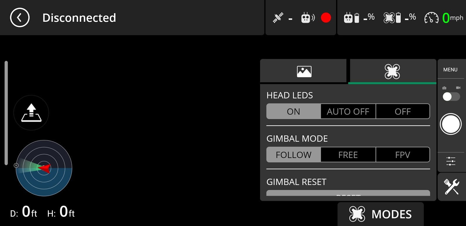
AT 409 Lab 1

 Lab 1 was an introductory lab to the Unmanned Aerial Systems Capstone Course. The projects for the UAS Capstone include:

1. Working in a mock up of a search and rescue operation
2. Evaluation of UAS platforms, sensor qualities and abilities
3. Comparing PPK Data with UAS data on differing platforms
4. Assessing how altitude can impact quality of data colleciton by sensor with UAS platforms
5. Mapping the entire Martell Forest
6. Changing colors of layers of the Martell Forest in order to classify and quantify levels of invasive honey suckle
7. Performing electric power line inspection in two person teams with M210 and Z30 sensors  

The Bramor C4EYE and the Matrice 210 are the two UAVs we will be using for the capstone project. The Bramor C4EYE is a fixed wing UAV. The Bramor was developed for military reconnaissance missions by C-Astral Aerospace in Slovenia. The version we use was tweaked for commercial purposes. The drone costs about $100,000 and is currently being used by the University for search and rescue research applications. The Bramor utilizes a catapult type launch system in order to facilitate take off and slows down for soft landings by using a parachute. The operation of the Bramor is completely autopilot and in emergency situations the failsafe is also the parachute. We were told about the importance of good crew resource management and organization while operating this UAV. A lot of emphasis was placed on using good communication between team members. Sometimes the app Zello is used to communicate during flights. They also use the 3 boxes that contain the Bramor to outline an area for flight operations and create a physical barrier. 

The multi-rotor UAV we will be using for the capstone is the DJI Matrice 210. The Matrice 210 is a quad rotor designed for commercial applications. It has a high quality zoom lens and a thermal camera. The zoom lens is called the Z30 and the thermal camera is the M210 sensor. During class we had the opportunity to operate both of these sensors. We learned how to use a transmitter with these sensors as well as switch between them while in flight. 

The camera settings for the Matrice 210 are as follows:

-shutter speed 1600

-fstop: 4.5

-ISO: 100

-35 mm lens

Lab 10: Measure Ground Control

Introduction:

Measure Ground Control is a SSoT for flight records, mission planning, and maintenance of UAS. An SSoT is defined as a single source of technology solution. Measure Ground Control was developed with the help of commercial drone operators with the purpose of being the most complete software program for drones. The application itself has a copious amount of useful features.

Measure Ground Control is capable of:

• creating and scheduling missions
• assigning pilots and equipment for missions
• creating a grid or way point flight plans
• making one aware of airspace and weather conditions
• requesting LAANC authorization
• flying GPS aided manual controls
• using track modes 
• automatically uploading flight logs
• storing unlimited imagery and flight logs
• accessing flight playback
• automatically flagging incidents
• managing equipment
• automatically tracking equipment usage

This SSoT is extremely efficient because it rids the need of using multiple applications at once. It can be easy to become unorganized and distraught during a UAS operation while switching between multiple apps and platforms. (At least it is for an amateur like myself.) This SSoT is also useful for mission planning and organization because it allows you to schedule as well as keep a calendar for missions. The ability to automatically update flight logs with great accuracy is also a perk when it comes to organization. 

There are also an immense amount of safety features available through this SSoT.  The ability to make phone calls to ATC through the app as well as request LAANC authorization is an incredibly useful feature for flight authorization. The ability to track equipment usage is also useful because it allows one to set a time window for when maintenance may be necessary. Accessing flight playback can be beneficial in regards to safety because it allows for pilots to determine errors in judgement that may have lead up to flight incidents or crashes. It almost goes without saying that the ability to determine weather anomalies and airspace requirements is also integral to maintaining safe UAS operation. 

Within this lab I will explore the mobile and desktop features of Measure Ground Control. I will use this application in order to determine airspace requirements, plan a mission, and explore the fly screen.

Methods:

(Figure 1: Purdue Wildlife Area Location)

The first thing I did before diving into the app was find the exact location/ address for the Purdue Wildlife Area. I participated in a lab for AT 309 at this location, so I believed it to be outside of class Delta airspace. I wanted to ensure this information was accurate, and the Purdue Wildlife Area is in fact in uncontrolled airspace. In this area normal CFR 14 Part 107 rules apply. The ceiling for the class G airspace could be 700-1200 ft AGL, but one would never legally reach this ceiling figure 2 below shows the class delta relative to an estimated location of the Purdue Wildlife Area. I later verified this again within the mission planning section of the application by inputting the address of the location. This can be seen in figure 3 below. 

(Figure 2: Approximate Purdue Wildlife Area Location)

(Figure 3: Verification that the area is outside of class D airspace) 

After verifying the airspace regulations for the Purdue Wildlife Area I decided to do the same for Martell Forest. The location for Martell Forest can be seen below in figure 4. Although the pin for Martell forest appears to be outside of the class Delta; it is hard to tell where the forest stops and ends. In order to be safe in this situation I would recommend recording GPS or ground control point locations in order to verify the mission will not take place within the class delta. If it is necessary for the mission to take place within classified airspace; one may have to acquire a waiver from the FAA and clear the flight with ATC. Requirements for airspace around this area can be seen in figure 6. Within the map section of the application it is also possible to view airspace advisories. These advisories can be seen in figures 7 and 8. 

(Figure 4 location of Martell Forest) 

(Figure 5 possibility that Martell may extend into classified airspace) 

(Figure 6 airspace information) 

(Figure 7 Airspace Advisories)

(Figure 8 Airspace Advisories) 

Figure 9 below shows the fly screen display on the mobile application. The fly screen is useful because the large amount of features rid the need for the use of multiple apps in order to do things like adjust gimbal and camera settings. This screen is used for pre determined flight plans or GPS assisted manual flight. 

(figure 9 flight screen display) 

Figure 10 shown below displays the flight planning section of the mobile application. I chose to plan a grid flight pattern over the Purdue Wildlife Area.  You can search for previous flight plan which can save time and create consistent results when operating in the same area. I also explored the mission planning section of the application which is incredibly useful for organizing missions because it allows you to do things like schedule the mission, clear the flight, organize equipment and assign pilots all in one page. There is also a terrain option within the flight planning screen. This setting is useful for safety because it allows for the drone to make slight adjustments to its altitude based off of the terrain that it is flying over. 

(figure 10: flight planning screen) 

Conclusion:  

After completing this lab activity I am convinced that Measure Ground Control SSoT is an incredibly useful and efficient tool for commercial UAS operation. I believe what sets this application apart from others is the strong emphasis on safety and mission planning in combination with the features available through the flight screen. I believe that an SSoT application like this is beneficial because it allows UAS operators to work through one application at a time. I'm interested in actually using this application for flight in the future. 

Lab 9: Using Arc Collector

Introduction:

Arc Collector is a mobile app that allows for the gathering of data within the field so that it can later be synchronized with other GIS data. Arc Collector allows you to collect GIS information in the field, collect location coordinates, and upload this information directly into a GIS database from a mobile device. The app allows for fieldworkers to complete tasks more accurately and efficiently. The purpose of the app is to reduce error as well as decrease the amount of time necessary in the field. The app uses GPS in order to edit map data and also to create points, lines, area features, and other vector data.

In this lab activity Arc Collector is used to map out a park area. I chose to map out the area outside of a Purdue University residence hall. Within the parks map it is possible to log the locations of objects like benches, trees, trash cans, restrooms and more. It also allows for you to log paths by streaming your location while walking along the path.

The tutorials used for this lab activity can be found here:

Part 1: https://www.esri.com/arcgis-blog/products/collector/field-mobility/try-collector/

Part 2: https://www.esri.com/arcgis-blog/products/collector/field-mobility/make-your-first-collector-map/

Methods Part 1: Collection

The first object that I "collected" was the bench/ table that I was using as a work station. It can be seen in figure 1 below. This was done by recording a GPS coordinate while near the table and taking a photo. Figure 2 shows the data associated with the table.

(Figure 1: Photo of the table)

(Figure 2: Table Information and Path Shown in Green)

After this was done I collected the data to map a path within the area. A photo of the path is shown below in figure 3. Figure 2 shows how the path appeared within the app after streaming. Paths are created within the app by streaming GPS information at multiple points while walking down the path. I collected a few other objects which can be seen below in figures 3-6. 

(Figure 3: V-Shaped Path)

(Figure 4: Tree) 

(Figure 5: Other Table) 

(Figure 6: Tree Information) 

Methods Part 2: Creating a Map: 

The first part of this process is to prepare a layer. The places layer is the first layer that needs to be configured. I decided to create a layer for paths as well. In the "My Content" the create button is selected, followed by selecting the feature layer tab in the drop down menu. From here the "build layer" button is selected. The default layers that are given include points lines and polygons. These default layers can be seen below in figure 7.  I changed the point layer into a places layer, and I also changed the lines layer into a path layer. I decided to delete the polygon layer. I proceeded to set the extent for my layer to cover the Purdue Campus. I then selected a title for the map. The extent area for the map is shown below in figure 8. 

(Figure 7: Default Feature Layers)

(Figure 8: Area for Map)

Once the layer is created it is necessary to make some adjustments within the data tab. Once navigating to the fields page within the data tab it is necessary to create two fields. The first field is "type of amenity" which is then categorized as an integer. An integer is defined as a number that can be written without a fraction or decimal. The second field that was created was called "notes" which was a string type of field. A string can be defined as a sequence of characters. These fields are shown below in figure 9 Within the "type of amenity field" a list is created. Numbers are assigned for a water fountain, a picnic table, and a restroom. Finally it is necessary to ensure that attachments are enabled on all of the layers. This is shown in figure 11. 

(Figure 9: Fields and Field Types)

(Figure 11: Enabling Attachments)

(Figure 12: Objects and paths collected)

Discussion: 

Overall I really enjoyed doing this lab. It was pretty cool to see some of the things that the arc collector app is capable of and before this I had no idea that an app like this existed. The ability to collect data with a mobile device and put it directly into a GIS database is a really interesting concept to me and I would be interested in finding out more applications of this software. I could see it being very useful for things like surveying and inspections. 

Lab 8: Value Added Data Analysis

Introduction:

UAS data that is gathered conscientiously can provide much more insight than what is seen at face value. Depending on the skills of the operator and analyst there can be a surprisingly copious amount of value that can be extracted from a UAS data set. This lab activity demonstrates this by providing instructions regarding how to classify aerial images in order to determine their surface types. Only the first two steps of this tutorial are necessary to complete for the lab activity. The instruction for this lab activity was originally a tutorial created by ESRI, and the full set of instructions can be found here:

https://learn.arcgis.com/en/projects/calculate-impervious-surfaces-from-spectral-imagery/

In this lab activity ArcGIS pro is used in order to classify surfaces as pervious or impervious. Pervious surfaces are those which allow water to pass through; whereas impervious surfaces do not allow water or liquid to pass through. Some examples of pervious surfaces related to this lab include bare Earth, grass, and water. Some examples of impervious surfaces related to this lab include roofs, driveways, and roads.

So, why would it be beneficial for one to be able to classify surfaces in this way? The tutorial actually provides a very clear example as to why this method of classifying surfaces is useful. Apparently many governments charge landowners that possess substantial amounts of impervious surfaces on their property. So, this method of classification could therefore be used in order to calculate these fees per parcel. In this situation a parcel can be defined as a specific plot of land. Examples of these parcels can be found below.

Methods:

Part 1: Segmenting the Imagery:
Before the imagery is classified it is necessary to adjust the band combination in order to see the different features with ease. In regards to aerial imagery a "band" is a layer within a raster data set.

(Figure 1: original map with parcels) 

Figure 1 above shows what the map looks like when it is originally imported into ArcPro. The area shown is a neighborhood in Louisville Kentucky. This is one of the areas that is known to charge fees for impervious surfaces. The yellow lines represent parcels or individual land lots. 

(Figure 2: Bands)

Figure 2 above shows the different band layers within the raster data set. 

(Figure 3: Extract Bands Function) 

Figure 3 shows the raster function that we will be using. In this case we will be using the "extract bands" function. Raster functions are used to apply an operation to an image "on the fly" this means that the original data remains unchanged. It also means that a new data set is not created. The output of this function takes the form of a layer that only exists within a specific project. The "extract bands" function is used in this case in order to create a new image with only three bands that will be used to tell the difference between pervious and impervious surfaces. 

(Figure 4: Extract Bands Parameters)

Figure 4 displays the parameters for the extract bands function. Band IDs is used as the method of identifying the bands because it is the most simplistic. Band ID's uses a single digit number in order to label each band. In this function we will be using band 4, band 1, and band 3. Band 4 is "near infrared" which focuses on vegetation. Band 1 is red and it focuses on vegetation as well as human-made objects. 

(Figure 5: Extract Bands Layer with Parcels) 

(Figure 6: Extract Bands Layer with no Parcels) 

After the extract bands function is run the layer created should look like Figures 5 and 6 shown above. The only difference between the two images is that the parcel layer is not visible in Figure 6. Within these images vegetation is red, roads are gray, and roofs tend to be displayed as gray or blue. The next step in the process involves using the classification wizard. 

 (Figure 7: Image Classification Configuration) 

 (Figure 8: Setting Output Location) 

Figures 7 and 8 shows the adjustment of parameters within the image classification wizard. The classification shcema is actually found by using the option "use default schema" within the drop down menu. The output location also needs to be changed to the "neighborhood data". The next step in this process is to segment the image. 

(Figure 8: Segmented Image Preview)

In order to segment the image a few adjustments must be made to the parameters spectral detail, spatial detail, and minimum segment size in pixels. 

Spectral detail is set to 8, spatial detail is set to 2, and minimum segment size is set to 20. If this Spectral detail determines the level of importance assigned to spectral differences between pixels from a scale of 1 to 20. If this value is high it means that pixels have to be more similar in order to get grouped with each other. This also creates a higher number of segments. Since impervious and pervious surfaces have very different spectral signatures a low value is used in this scenario.

Spatial detail determines the level of importance assigned to the proximity between pixels again, on a scale of 1 to 20. A high value on this scale indicates that pixels must be closer to each other in order to be grouped together.  

Segment size is not determined on a scale of 1 to 20. Segments with less pixels will be merged with neighboring segments. In this situation you don't want the segment size to be unreasonably small, but you also don't want to have impervious and pervious segments merged together. Once these settings are adjusted appropriately the map should look like figure 8 shown above. 

 (Figure 9: first training sample) 

The next step in this process is to create training samples so that the imagery can be further classified into specific pervious and impervious surfaces. This is done by first creating two primary classes; impervious and pervious. Within these two categories there will be more specific individual classes. Impervious classes were created for roofs, roads, and driveways. Pervious classes were created for bare Earth, grass, water and shadows. 

Once these sub classes are created training samples are created by drawing polygons on these objects so that the software can learn to identify them. Once the polygons are created for a single class they must be collapsed together. Figure 9 shows the first training sample created. Figure 10 displays more training samples for identifying gray roofs. Figure 11 shows several different types of training samples. 

(Figure 10: More roof training samples) 

(Figure 11: Different types of training samples) 

The final step in this process is classifying the image. In order to do this the classifier tool must be set to the "support vector machine" and the maximum number of samples per class must be set to zero. This second step ensures that all of the training samples are used. 

Once these parameters are adjusted the classification is ran and the resulting image should look like figure 12 below. The image below actually has a couple of errors in classification. A good example of this would be the pond in the lower left corner. These anomalies can be reclassified manually using polygons.  

(Figure 12)

Lab 6: Processing Pix4D Imaging with GCPs

Introduction:

Ground control points (GCPs) are markers with known coordinates used in aerial imaging. Ground control points are useful because their known coordinates can be used as a reference in order to accurately map large areas. Ground control points are often square shaped markers like the one shown below in figure 1. Ground control points need to be easily recognizable. They are often black and white, patterned, or made with other high contrast colors. 

                                                  (Figure 1: GCP Example)

The purpose of this lab was to process the same imagery from lab 4, but this time ground control points are used in order to improve accuracy. 

Methods Part 1: Importing the GCP Data

The first step in this process was to import the GCP data into pix4D. Once this is accomplished it is necessary to ensure that the output coordinate system and the coordinate system used for the ground control points are the same. Figure 2 below shows the selection of the appropriate coordinate system. The coordinate system used for this lab was the world geodetic system 1984. In order to correctly match the output coordinate system to the coordinate system used to collect the GCPs you can check the meta data.  It is also necessary to make sure that the appropriate camera model is selected and the linear rolling shutter setting is selected. Figure 3 below shows the adjustment of the camera model settings. 

 (Figure 2: Matching Output Coordinate Systems to GCPs)

(Figure 3: Adjusting Camera Settings)

Methods Part 2: Processing the GCP Data

Once again the processing will be done in two separate parts. Initial processing is done separately from the generation of the point cloud and orthomosaic. Before this step it is important to make sure that certain settings regarding the GCP coordinates are correct. GCPs can be displayed in XYZ or YXZ format. In this case it is necessary to adjust the settings to YXZ. Figure 4 shows the adjustment of this setting. After slightly adjusting some more intial processing options initial processing can begin. After initial processing is complete a quality report is generated. 

(Figure 4: Setting the correct coordinate order)

Methods Part 3: Marking and Optimizing

After initial processing is finished its necessary to make sure that the GCP's are as accurate as possible. This is accomplished by adjusting the location of a digital pointer/marker so that it lines up as close as possible to the center of the actual GCP. Figure 5 shows the overall process of correctly marking the GCPs. Figure 6 shows a close up of locating the actual GCP within the imagery. Figure 7 shows the difference between the GCPs before and after optimization. It is important to put the marker directly over the center of the angle. GCPs can be slightly more accurate when they are manufactured like the one in figure 1 above. However when making a temporary or painted GCP it is important to note that X shapes are often less accurate than L shapes. After the GCPs are marked steps 2 and 3 of the processing can be completed. The DSM and orthographic can then be generated. 

(Figure 5: Optimizing GCPs)

(Figure 6: Setting the pointer over the center of the angle/ Locating the GCP within the imagery)

(Figure 7: Difference between GCPs before and after they are optimized) 

Methods Part 4: Layout Maps and Comparisons:

Figure 8 Below shows a layout map made from data with GCPs. Figure 9 shows a layout map made from data without GCPs. As you can see there is a very significant difference in accuracy between the two. You can tell from the surrounding topography that the orthomoasic with GCPs is superior. An easy way to quickly realize this is to look at how out of place the pond near the top of the image is in figure 9. Figure 10 is an animation created using screenshots from arcGIS pro it was made by fading the two maps over one another in order to showcase the difference in the location with and without ground control points. 

(Figure 8 Accurate GCPs Map)

(Figure 9 No GCPs)

(Figure 10 Maps overlaid with Transparency)

Conclusion:

Ground control points are necessary in order to create accurate maps using aerial imagery. They provide a reference point with known coordinates in order to align the imagery with a coordinate system. It is important to make sure that the coordinate system used to collect the GCPs is the same as the output before processing. After completing this lab I feel that I now have an understanding of how GCPs are placed, how their coordinates are recorded, and how they are used within software to create geographically accurate maps. 

Lab 5: Living Atlas

Introduction:

Living Atlas is a tool created by ESRI that allows access to an extensive library of geo-spatial data. This data can easily be added to maps in ArcGIS pro using the catalog tab. In this lab we learned how to easily find content within the living atlas, how to view the data online, how to import the data into ArcGIS pro, how to adjust settings to display data from specific times, how to view charts and graphs of the data, how to configure the data in the most optimal way, and how to use the data to create proper layout maps. This tutorial is relevant to unmanned aerial systems because I believe it would be extremely useful in some cases to supplement data collected by UAS with already existing data. It would also allow one to supplement UAS data with other information in real time. 

5 lessons that are of interest:

1. https://learn.arcgis.com/en/projects/investigate-pollution-patterns-with-space-time-analysis/

This tutorial involves working with global pollution data. The purpose of the tutorial is to find differences in pollution patterns by relating them to space and time. By the end of the tutorial one would be able to find areas with extreme or abnormal pollution patterns. This lesson is interesting to me because it is related to environmental sustainability.   2. https://learn.arcgis.com/en/paths/combating-crime-with-gis/

This tutorial involves tracking incidents related to prescription drug abuse, graffiti, and card fraud. This data is then used in a way that assists law enforcement in the future. This tutorial is interesting to me because I wouldn't normally expect geo-spatial data to be used in order to stop crime. 

3. https://learn.arcgis.com/en/paths/using-lidar-data-in-arcgis-pro/

This lesson teaches one basics about lidar data, how to create a LAS datasheet, how to take measurements using LAS datasheets, creating mosaic data-sets, creating hill shades, and exporting contours. I think that this tutorial is extremely relevant to UAS because lidar data is used in so many UAS applications. 

4. https://www.esri.com/content/dam/esrisites/en-us/media/pdf/learn-arcgis/find-fish-in-the-bering-sea.pdf

This lesson teaches you how to map ocean temperatures, build prediction surfaces, and compare cross validation errors to determine which prediction surfaces are the most accurate. The objective is to use this data to find fish in the Bering Sea. I find this tutorial interesting because I enjoy applications of GIS data that relate to wildlife and sustainability. 

5. https://learn.arcgis.com/en/paths/try-machine-learning-with-arcgis/

This lesson walks you through several machine learning applications involving alternate climate zones, using deep learning to assess tree health, and using AI to downscale climate data. This tutorial is interesting to me because I am curious how artificial intelligence can be used with GIS data. 

Methods Part 1: Exploring the Living Atlas Website

During this portion of the lab we learned how to filter through the living atlas website in order to locate specific data-sets. We use filters in order to find an item named "GLDAS Soil Moisture 2000 – Present". Figure 1 shows how this data-set looks within the online map viewer. 

(Figure 1)

We then dive deeper into the information presented using the living atlas application. First, we locate a specific location using coordinates and find the Grand Ethiopia Renaissance Dam. Once this location is selected we can use the app in order to showcase different graphs displaying data about this specific location. Figure 2 below is an example of one of the graphs, and it specifically displays the soil moisture in the area. 

(Figure 2)

Methods Part 2: Use Living Atlas in ArcGIS Online

The first step in this portion of the lab is to create a base map. In this case we use the light gray canvas as the base. Next, we browse living atlas to find a layer titled "USA NLCD Land Cover". Once this layer is added we focus on Las Vegas, Nevada. This layer can be seen in figure 3 below. We then use the time slider in order to view data collected from different years and observe how the data changes.We then use a renderer in order to only display data for developed land, and then we adjust the symbology of the data.

(Figure 3)

Methods Part 3: Use Living Atlas in ArcGIS Pro

For this portion of the lab we use an existing data-set that contains information about hurricane Irma. We download this data and then import it into ArcGIS pro. We then use the portal in the catalog pane in order to add the data to our map. Once the data is added to the map several layers become available as shown in figure 4. We then use this data to perform analysis in the Geo-Processing pane. Using a forecasting cone we find that 3,523 nursing homes that may be at risk from this hurricane.

(Figure 4)

Methods Part 3: Creating Maps Using Living Atlas 

The first map I created shown in Figure 5 displays minor weather events and othe minor advisories in the united states in real time. The data-set used to create this map had several other layers that included more severe conditions, but I chose to create a map that only displayed minor events.

(Figure 5)

The second map shown below in figure 6 displays the crime index in the state of South Carolina. The crime index is displayed using shades of red to represent each county's crime rate relative to the national average. Since this data-set is organized by county I chose to showcase an individual state, and South Carolina displayed a diverse spectrum. 

(Figure 6)

My third map used a data layer describing data from wind/ weather stations in the United States. The data is displayed using arrows that represent wind direction and intensity.

(Figure 7)

The fourth map I created shows the density of roads within the United States. The lighter the color displayed on the map the more roads can be found within that area. 

(Figure 8)

The final map shown below showcases the risk for Earthquakes within the United States. It ranks areas on a scale of 0-100; 0 being the lowest risk for earthquakes and 100 being the highest. I made this layer semi-transparent so state borders can still be observed. 

Conclusion: 

Living Atlas is an extremely useful library of data that can be used within ArcGIS pro. Living Atlas can be used to display data in real time as well as data from the past. This large collection of data would be extremely useful if it is used in conjunction with data collected by UAS.